
Battle of the Programming Languages: R vs Python
We are going to compare Functions exist in both R and Python for same operations. And for this we took the Titanic dataset which contains the Passenger details.
Importing a CSV
Reading Data in both the languages is similar, but the only difference is for python we have to import pandas library for reading the Data. Once the importing is done we can look into the data by applying the below functions.
| R | Python |
| titanicimport pandas as pd titanic = pd.read_csv("train.csv") |
Dimension and Shape
If we want to look the Dimension of the above imported Data. You can get it from the below functions.
| R | Python |
| dim(titanic) | titanic.shape |
| [1] 891 12 | (891, 12) |
The above code brings you the number of passengers in titanic ship and the number of columns present in data.
Head and Tail
If you want to see some of the data like top rows (Any number of rows by default it gets 5 rows) or bottom rows form the Data frame. There are functions in similar functions in both R and Python.
| R | Python |
| head(titanic,2) | titanic.head(2) |
| PassengerId Survived Pclass 1 1 0 3 2 2 1 1 |
PassengerId Survived Pclass 0 1 0 3 1 2 1 1 |
| tail(titanic,2) | titanic.tail(2) |
PassengerId Survived Pclass 890 890 1 1 891 891 0 3 |
PassengerId Survived Pclass 889 890 1 1 890 891 0 3 |
Here head and tail functions applied on Titanic dataset to look at the first two rows of Data. If you observe clearly the index values are different in both R and Python. It is because Python index starts with '0'.
Basic Statistics of Data (Summary and Describe)
| R | Python |
| summary(titanic) | titanic.describe() |
| PassengerId Survived | PassengerId Survived |
| Min. : 1.0 Min. :0.0000 1st Qu.:223.5 1st Qu.:0.0000 Median :446.0 Median :0.0000 Mean :446.0 Mean :0.3838 3rd Qu.:668.5 3rd Qu.:1.0000 Max. : 891.0 Max. :1.0000 |
count 891.000000 891.000000 mean 446.000000 0.383838 std 257.353842 0.486592 min 1.000000 0.000000 25% 223.500000 0.000000 50% 446.000000 0.000000 75% 668.500000 1.000000 max 891.000000 1.000000 |
The above two functions are for determining some basic statistics column wise. Whereas python gives two more statistic values compared to R function. The main difference between these functions is R contains Separate functions and for Python we have to call the required methods on the Data as it is more of object oriented type programming.
Slicing the Data
| titanic[1:5,1:3] | titanic.iloc[0:5,0:3] |
| PassengerId Survived Pclass 1 1 0 3 2 2 1 1 3 3 1 3 4 4 1 1 5 5 0 3 |
PassengerId Survived Pclass 0 1 0 3 1 2 1 1 2 3 1 3 3 4 1 1 4 5 0 3 |
Sub setting Data
Here in this case for sub setting the Data I took only some columns from the titanic Dataset. For the convenience of displaying the output.
Using sam_data sam_data = titanic[['PassengerId', 'Survived','Sex','Age']] for Python
I created sam_data for applying subset function.
| subset(sam_data,Survived == 1& Sex == 'male') | sam_data[(sam_data.Sex == 'male') & (sam_data.Survived ==1)].head(2) |
| PassengerId Survived Sex Age 18 18 1 male NA 22 22 1 male 34 24 24 1 male 28 37 37 1 male NA 56 56 1 male NA 66 66 1 male NA |
PassengerId Survived Sex Age 17 18 1 male NaN 21 22 1 male 34.00 23 24 1 male 28.00 36 37 1 male NaN 55 56 1 male NaN 65 66 1 male NaN |
The important thing here is the representation of NA in Python is NaN.
Ordering the Data
We ordered the Sample Dataset By
| arrange(sam_data, Survived, desc(Age)) | sam_data.sort_index(by=['Survived', 'Age'], ascending=[True, False]) |
| PassengerId Survived Sex Age 1 852 0 male 74.0 2 97 0 male 71.0 3 494 0 male 71.0 4 117 0 male 70.5 5 673 0 male 70.0 6 746 0 male 70.0 |
PassengerId Survived Sex Age 851 852 0 male 74.0 493 494 0 male 71.0 96 97 0 male 71.0 116 117 0 male 70.5 672 673 0 male 70.0 745 746 0 male 70.0 |
Joins
For Performing join operations we created three different data frames from the titanic Dataset
df_Survived df_Sex df_Age
df_Survived = sam_data[['PassengerId', 'Survived']]
df_Sex = sam_data [['PassengerId', 'Sex']]
df_Age = sam_data [[ 'PassengerId', 'Age']]
| Inner Join |
Table_Inner_J = merge ( merge(df_Survived, df_Sex, key = "PassengerId" ), df_Age , key = "PassengerId") |
Table_Inner_J = pd.merge ( pd.merge(df_Survived, df_Sex, on = "PassengerId" , how = "inner" ), df_Age , on = "PassengerId" , how = "inner") |
| Outer Join | Table_Outer_J = merge ( merge(df_Survived, df_Sex, key = "PassengerId" , all =TRUE), df_Age , key = "PassengerId", all = TRUE) |
Table_Outer_J = pd.merge ( pd.merge(df_Survived, df_Sex, on = "PassengerId" , how = "outer"), df_Age , on = "PassengerId", how = "outer") |
| Left Join |
Table_Left_J = merge ( merge(df_Survived, df_Sex, key = "PassengerId" , all.x =TRUE), df_Age , key = "PassengerId", all.x = TRUE) |
Table_Left_J = pd.merge ( pd.merge(df_Survived, df_Sex, on = "PassengerId" , how = "left"), df_Age , on = "PassengerId" , how = "left") |
| Right Join |
Table_Right_J = merge ( merge(df_Survived, df_Sex, key = "PassengerId", all.y = TRUE), df_Age , key = "PassengerId", all.y = TRUE ) |
Table_Right_J = pd.merge ( pd.merge(df_Survived, df_Sex, on = "PassengerId" , how = "right"), df_Age , on = "PassengerId" , how = "right") |
The major Difference in R and Python for joining operation is both can be done using merge function. But for python we have to import pandas library for using the merge function to perform these join functions. We can join three Data frames at a time by applying merge function two times.
Missing Values Treatment:
In Missing Values treatment first thing we have to do is identify the NA values by running the first block of code in below table. After getting the variables where missing values are there then you can impute them with the mean value of that respective column.
Here, second block of code replaces the NA values with the respective mean values.
| tail(is.na(sam_data)) | sam_data.isnull().tail() |
| PassengerId Survived Sex Age [886,] FALSE FALSE FALSE FALSE [887,] FALSE FALSE FALSE FALSE [888,] FALSE FALSE FALSE FALSE [889,] FALSE FALSE FALSE TRUE [890,] FALSE FALSE FALSE FALSE [891,] FALSE FALSE FALSE FALSE |
PassengerId Survived Sex Age 886 False False False False 887 False False False False 888 False False False False 889 False False False True 890 False False False False |
| sam_data["Age"][is.na(sam_data["Age"])]meanAge = np.mean(sam_data.Age) sam_data.Age = sam_data.Age.fillna(meanAge) |
|
| PassengerId Survived Sex Age [886,] FALSE FALSE FALSE FALSE [887,] FALSE FALSE FALSE FALSE [888,] FALSE FALSE FALSE FALSE [889,] FALSE FALSE FALSE FALSE [890,] FALSE FALSE FALSE FALSE [891,] FALSE FALSE FALSE FALSE |
PassengerId Survived Sex Age 886 False False False False 887 False False False False 888 False False False False 889 False False False False 890 False False False False |
Plotting the Data:
Python:
Import seaborn and matplot libraries for plotting the titanic dataset.
import matplotlib.pyplot as plt
import seaborn as sns
fig, (axis1,axis2) = plt.subplots(1,2,figsize=(10,5))
sns.countplot(x='Embarked', data=titanic, ax=axis1)
sns.countplot(x='Survived', hue="Embarked", data=titanic, order=[1,0], ax=axis2)
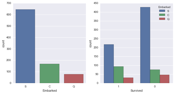 |
Here by using the subplots function from matplot package assigning space for two different graphs in single row. If we want to display two graphs in two rows each we have to assign a (2, 2) matrix as subplot.
R:
Using Par function, we will split the graph display into 1* 2 matrix
par(mfrow = c(1,2))
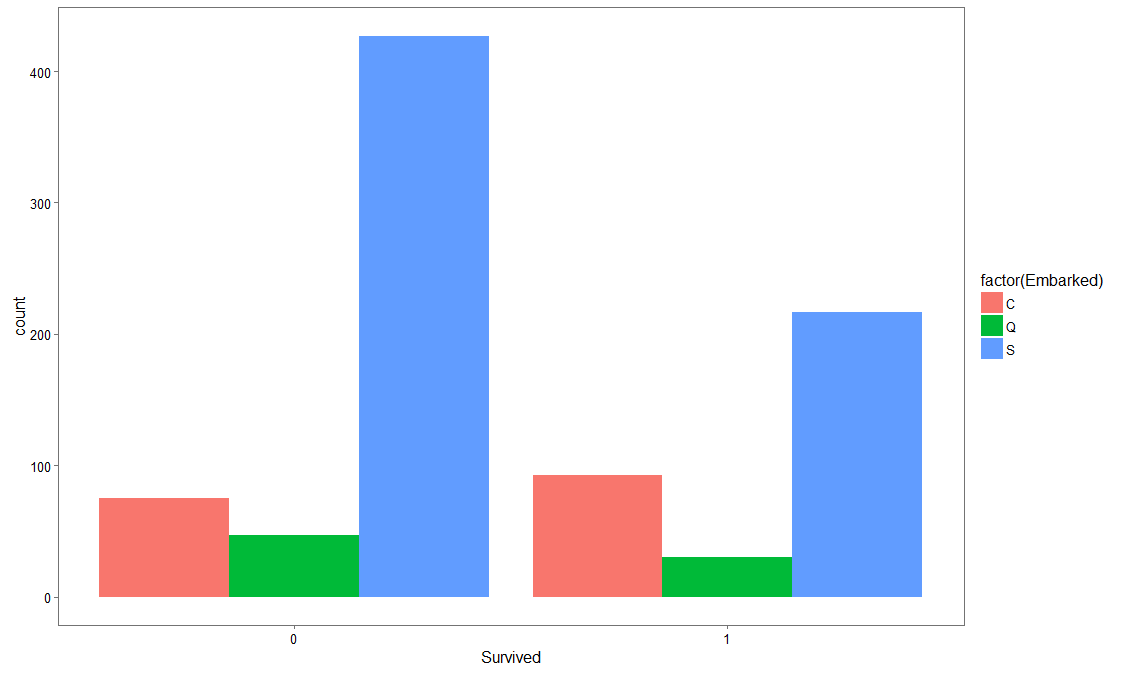
Below is the ggplot for first graph displayed below.
ggplot(titanic, aes(x = Survived, fill = factor(Embarked))) +
geom_bar(stat='count', position='dodge') +
scale_x_continuous(breaks=c(0:10)) +
labs(x = 'Survived') +
theme_few()
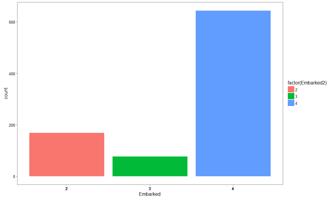
We are converting embarked column into numeric to plot its count using ggplot.
titanic$Embarked2
ggplot(titanic, aes(x = Embarked2))+
geom_bar(stat='count', position='dodge') +
scale_x_continuous(breaks= titanic$Embarked2) +
labs(x = 'Embarked') +
theme_few()
 |
 |
About Rang Technologies:
Headquartered in New Jersey, Rang Technologies has dedicated over a decade delivering innovative solutions and best talent to help businesses get the most out of the latest technologies in their digital transformation journey. Read More...